set.seed(194)

# Generate Data
n <- 2000
p <- 10
X <- matrix(rnorm(n * p), n, p)
X.test <- matrix(0, 101, p)
X.test[, 1] <- seq(-2, 2, length.out = 101)

W <- rbinom(n, 1, 0.4 + 0.2 * (X[, 1] > 0))
prob  <- 0.4 + 0.2 * (X[, 1] > 0)
Y <- pmax(X[, 1], 0) * W + X[, 2] + pmax(X[, 3], 0) + rnorm(n)

###################################
###################################
#
#
# 1. estimate m(X) and e(X)
#    using cross-fitting
#
###################################
###################################

# cross-fitting index
K  <- 10 # total folds
ind  <- sample(1:length(W), replace = FALSE, size = length(W))
folds  <- cut(1:length(W), breaks = K, labels = FALSE)
index  <- matrix(0, nrow = length(ind) / K, ncol = K)
for(f in 1:K){
    index[, f]  <- ind[which(folds == f)]
}

# Build a function to estimate conditional means (m(x) and e(x)) using random forest
fun.rf.grf  <- function(X, Y, predictkfold){
    rf_grf  <- regression_forest(X, Y, tune.parameters = "all")
    p.grf  <- predict(rf_grf, predictkfold)$predictions
    return(p.grf)
}

# storing
predict.mat  <- matrix(0, nrow = nrow(index), ncol = K) # to store e(x)
predict.mat2  <- predict.mat # to store m(x)


# for each fold k use other folds for estimation

for(k in seq(1:K)){
    predict.mat[, k]  <- fun.rf.grf(X = X[c(index[, -k]), ], Y = W[index[, -k]], predictkfold = X[c(index[, k]), ])
    predict.mat2[, k]  <- fun.rf.grf(X = X[c(index[, -k]), ], Y = Y[c(index[, -k])],
                        predictkfold = X[c(index[, k]), ])
}

W.hat  <- c(predict.mat)
Y.hat  <- c(predict.mat2)

################################
################################
#
# 2. Use LASSO to minimize
#    the loss function
################################
################################

# rearrange features and response according to index
XX  <- X[c(index), ]
YY  <-  Y[c(index)]
WW  <- W[c(index)]

resid.Y  <-  YY - Y.hat
resid.W  <- WW - W.hat

# Create basis expansion of features
for(i in seq(1, ncol(XX))) {
    if(i == 1){
        XX.basis  <- bs(XX[, i], knots = c(0.25, 0.5, 0.75), degree = 2)
    }else{
        XX.basisnew  <- bs(XX[, i], knots = c(0.25, 0.5, 0.75), degree = 2)
        XX.basis  <- cbind(XX.basis, XX.basisnew)
    }
}

resid.W.X  <-  resid.W * XX.basis
resid.W.X  <- model.matrix(formula( ~ 0 + resid.W.X))
#plot(XX[ ,1], pmax(XX[ , 1], 0))

# cross validation for lasso to tune lambda
lasso  <- cv.glmnet(
    x = resid.W.X,
    y = resid.Y,
    alpha = 1,
    intercept = FALSE
)

#plot(lasso, main = "Lasso penalty \n \n")

# lambda with minimum MSE
best.lambda  <- lasso$lambda.min

lasso_tuned  <- glmnet(
    x = resid.W.X,
    y = resid.Y,
    lambda = best.lambda,
    intercept = FALSE
)

#print(paste("The coefficients of lasso tuned are:", coef(lasso_tuned), sep = " "))
pred.lasso  <-  predict(lasso, newx = XX.basis)


#########################
#
# Causal Forest
#
#########################

X.test  <- matrix(0, nrow = nrow(X), ncol = ncol(X))
X.test[, 1]  <- seq(-3, 3, length.out = nrow(X))

tau.forest  <- causal_forest(X, Y, W)
tau.forest
tau.hat <- predict(tau.forest, X.test)$predictions
par(oma=c(0,4,0,0))
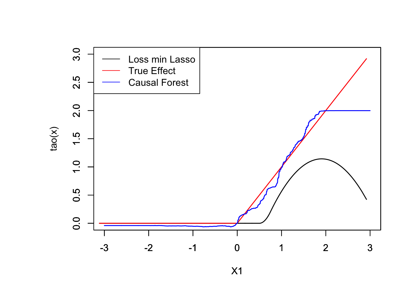
plot(XX[order(XX[ , 1]), 1], pred.lasso[order(XX[, 1])], ylim = c(0, 3), t = "l", xlab = " ", ylab = " ", xlim = c(-3, 3), lwd = 1.5)
par(new = TRUE)
plot(XX[order(XX[, 1]), 1], pmax(XX[order(XX[, 1]), 1], 0), col ="red", ylim = c(0, 3), t = "l", xlab = "X1", ylab = "tao(x)", xlim = c(-3, 3), lwd = 1.5)
par(new = TRUE)
plot(X.test[order(X.test[, 1]), 1], tau.hat[order(X.test[, 1])], t = "l", col = "blue", ylim = c(0, 3), xlab = "X1", ylab = "", xlim = c(-3, 3), lwd = 1.5)
legend("topleft", c("Loss min Lasso", "True Effect", "Causal Forest"), col = c("black", "red", "blue"), lty = rep(1, 3))