4.6 Estimation

There are different ways to estimate a regression specification. These include the method of moment estimation (as we’ve seen before), the maximum likelihood estimation (MLE), and computation estimation. Here, we take a look at the computational approach.

Let’s take a look at the error term, \(\epsilon_i\), a bit more carefully. We can flip the terms around and end up with.

\[\begin{equation} \epsilon_{i} = Y_{i} - (\alpha + \beta X_{i}) \tag{4.3} \end{equation}\]

Note that \(Y_{i} - (\alpha + \beta X_{i})\) are also termed as residuals.

Intuitively, we’d want to minimize the prediction error, right? Hence, we’d want to go for the estimates for \(\alpha\) and \(\beta\) such that these estimates minimize the residual sum of the squares (RSS). This gives us an objective function.

\[\begin{equation} \underbrace{min}_{\alpha, \; \beta} \sum_{i = 1}^N \bigg(Y_{i} - (\alpha + \beta X_{i})\bigg)^2 \tag{4.4} \end{equation}\]

The estimates of \(\alpha\) and \(\beta\) are termed as \(\widehat{\alpha}\) and \(\widehat{\beta}\), respectively.

Next, we’ll write an algorithm to follow the objective function.

1. Create a grid form for \(\alpha\) and \(\beta\) values.

alpha_vals  <- seq(18000, 35000, by = 10) 
beta_vals  <-  seq(500, 5000, by = 10)

# create a grid 
grid  <- expand.grid(alpha_vals = alpha_vals, beta_vals = beta_vals)

store  <- rep(0, nrow(grid))

2. Declare the objective function. The function takes in the values of \(X\), \(Y\), \(\tilde{\alpha}\), \(\tilde{\beta}\) and gives the ssr.

fun_objective  <- function(alpha, beta, X, Y) {

    # @Arg alpha: intercept
    # @Arg beta: slope
    # @Arg X: independent variable 
    # @Arg Y: dependent variable 

    residual_sq  <-  (Y - alpha - beta * X)^2
    ssr  <- sum(residual_sq)

    return(ssr)   

}

3. Pick the estimates on \(\alpha\) and \(\beta\) that minimizes the ssr.

for(i in seq(nrow(grid))){
store[i]  <- fun_objective(alpha = grid[i,1], beta = grid[i,2], X = educ, Y = income)
}

index  <- which(store == min(store))
coef  <- grid[index, ]

4. Compare the estimate that minimizes the ssr with estimates produced from in-built regression library in R.

print(grid[index, ])

##        alpha_vals beta_vals
## 258019      29670      2010

print(lm(income ~ educ, dat))

## 
## Call:
## lm(formula = income ~ educ, data = dat)
## 
## Coefficients:
## (Intercept)         educ  
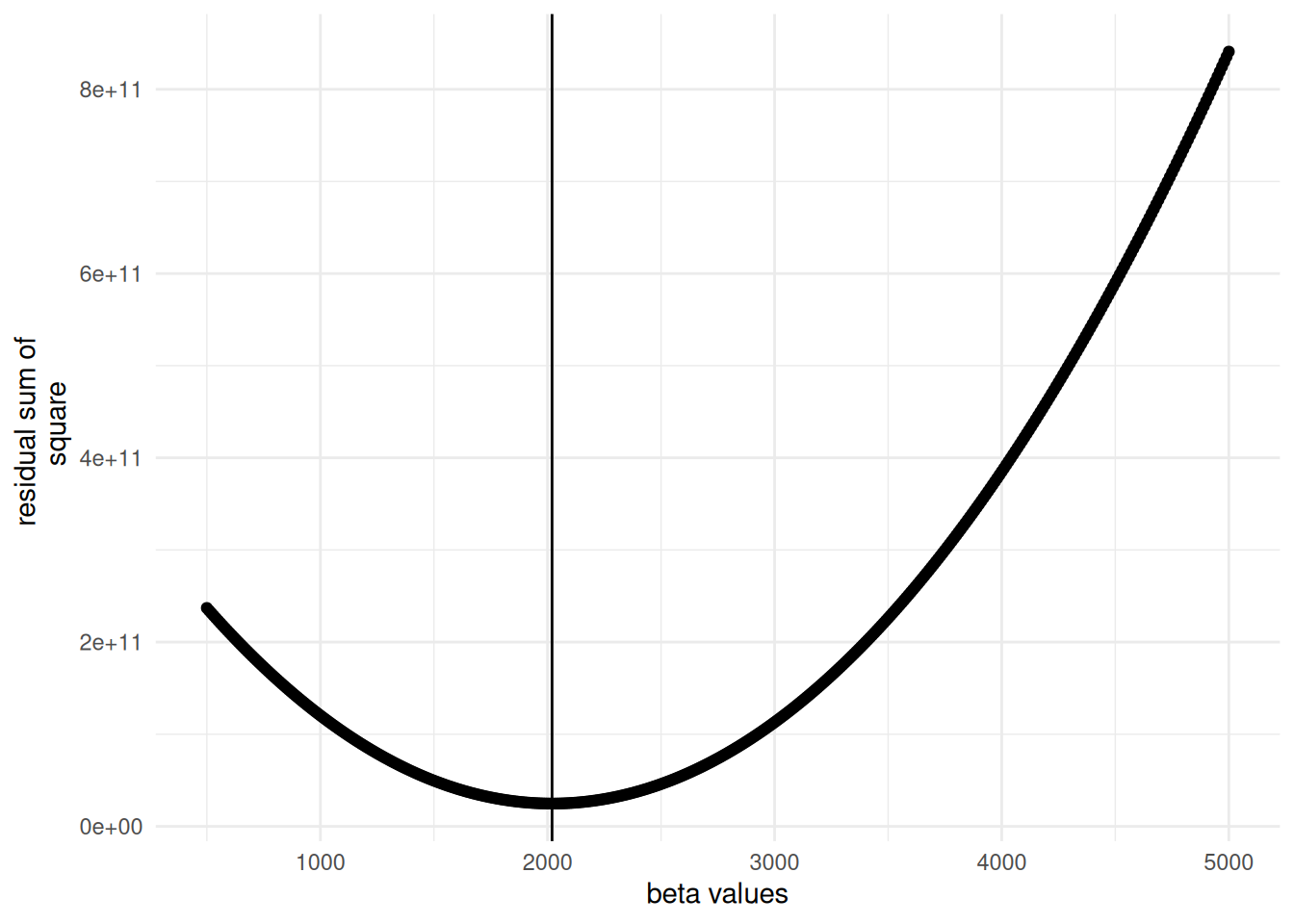
##       29650         2012

5. Let’s plot to see how ssr varies with estimates of \(\beta\). Fix the value of \(\alpha\) at the estimate from 4.

# create a dataframe
data  <- cbind(grid, store)

# restrict the value of alpha at the one that minimizes the ssr
data  <- data  %>% 
            filter(alpha_vals == coef[[1]])

# get the estimate on beta for the set alpha so that it minimizes ssr  
beta_hat  <- beta_vals[which(data$store == min(data$store))]

#plot
ggplot(data, aes(x = beta_vals, y = store)) + geom_point() + 
geom_vline(xintercept = beta_hat) + 
ylab("residual sum of \n square") + xlab("beta values")