4 Regression and Gradient Descent
Course: Causal Inference
Topic: Estimation of linear regression model with and without closed-form solutions
Last time we took a look at the method of minimizing the sum of the square of residuals. Today let’s take a look at two other ways of estimating a linear regression specification: i) Normal equation method, and ii) Gradient descent. We’ll do these manually and compare our results using python libraries to see whether we’ve done it correctly.
Lets first load the necessary libraries.
import numpy as np
import matplotlib.pyplot as plt
from sklearn.datasets import make_regression
from sklearn.preprocessing import add_dummy_feature
from sklearn import linear_model
import statsmodels.api as sm
root_dir = "/home/vinish/Dropbox/Machine Learning"
sklearn is an open sourced library in python that is mainly built for predictive data analysis, which is built on top of NumPy, SciPy, and matplotlib. You can get more information about this package on sklearn.
We’ll be using simulated data from sklearn’s module called “datasets” by using the make_regression() function. The true model has the following
attributes:
i) 2 informative features (X)
ii) 1 target (Y)
iii) intercept with the coefficient of 10
Let’s use make_regression() to simulate our data.
X, y, coefficient = make_regression(n_samples = 1000,
                       n_features = 2,
                       n_informative = 2,
                       n_targets = 1,
                       noise = 1,
                       bias = 10,
                       random_state = 42,
                       coef = True

)
Note that I’ve set coef = True. This will return the model parameters and the intercept is set at 10.
We take a look at the first five rows.
print features: [[-0.16711808  0.14671369]
 [-0.02090159  0.11732738]
 [ 0.15041891  0.364961  ]
 [ 0.55560447  0.08958068]
 [ 0.05820872 -1.1429703 ]]
target: [ 3.24877735  8.66339401 19.45702327 31.55545159  3.92293402]
And let’s print out the model parameters. Note these are the true coefficients that are used to generate data.
coefficients: [40.71064891 6.60098441]Plot the relationship between \(X1\) and \(Y\).
plt.figure(figsize=(8, 5))
plt.scatter(X[:,1], y)
plt.show()
#plt.savefig(root_dir + "/Codes/Output/make_data_scatter.pdf")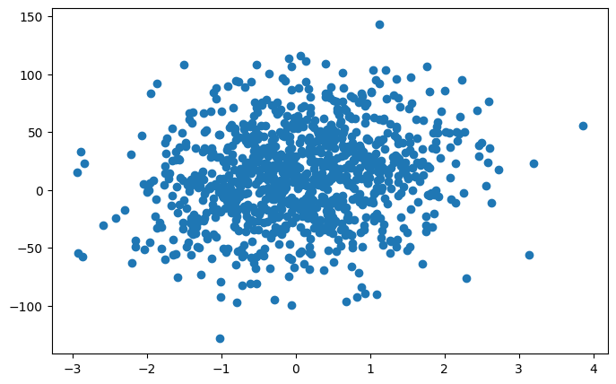
Now, we are ready to discuss two methods. Let’s start with the Normal equation method.
i. Normal Equation
Consider the following regression model specification:
\[ Y_i = \alpha + \beta_1 X_{1i} + \beta_2 X_{2i} + \epsilon_i \]
The job is to estimate model parameters \(\alpha\), \(\beta_1\), and \(\beta_2\).
Note that \(\epsilon_i\) is the error term and we’d want to minimize some version of this. Let’s write out the error as:
\[ \epsilon_i = Y_i - \alpha - \beta_1 X_{1i} -\beta_2 X_{2i} \]
We know that the error term \(\epsilon\) is a \(n \times 1\) vector. We can obtain residuals by using estimates of model parameters. Of course, we don’t want to pick any parameters – the estimates should follow some objective.
One idea is to estimate the model parameters with an objective of minimizing the mean of the error. However, this is 0 by construction. So what we’d want to do instead is minimize the mean squared error.
\[ MSE(X, h_{\theta}) = \frac{1}{m} \sum_{i=1}^{m} (\theta^{T} x_i - y_i)^2 \]
From the equation above, we know that the MSE is just the mean of the sum of the squared errors. We can write the sum of the squared of errors using the matrix version as:
\[ SSE(X, \theta) = (y - X\theta)^T(y-X\theta) \]
Expanding this and setting the derivatives w.r.t. \(\theta\) equal to zero gives: \[ \begin{aligned} SSE(X, \theta) = y^Ty - 2\theta^{T} X^Ty + \theta^{T}X^{T}X\theta \\ \frac{\partial(SSE)}{\partial{\theta}} = -2X^{T}y + 2X^{T}X\theta = 0 \end{aligned} \]
Now solving for \(\theta\) gives the normal equation: \[ \hat{\theta} = (X^TX)^{-1}X^{T}y \]
Let’s code the normal equation and print out the estimates. Before jumping into estimating the normal equation, we’ve got to be careful and add the intercept term (all ones) on X as the simulated data from make_regression comes without it. We’ll do this using add_dummy_feature() in sklearn.
# The normal equation
X = add_dummy_feature(X)
theta_best = np.linalg.inv((X.T @ X)) @ (X.T @ y)
print(f"coefficients from normal equation: {theta_best}")
coefficients from normal equation: [10.00156877 40.74650082 6.62076534]ii. Gradient Descent
Imagine that you are standing at the top of a mountain and want to descend the mountain as quickly as possible. One simple way is to consider a few directions – north, south, east, and west – and evaluate the steepness (gradient). Then you’d want to take a small step towards the steepest direction, pause, and re-evaluate the steepness. Doing this repeatedly gets you to the bottom of the mountain as fast as possible.
The idea of gradient descent is similar in context to the aforementioned analogy. We’ve already been exposed to the idea of MSE and the objective of minimizing MSE. Instead of using the closed form normal equation to solve for the minimum of MSE, gradient descent uses gradient of MSE to adjust the estimates and move closer to the minimum.
The gradient is a vector of partial derivatives of MSE that points to the direction of steepest increase increase in MSE. Hence, to minimize the loss, we’d want to move in opposite direction of the gradient. By repeatedly updating our parameter in this way, we move closer and closer to the minimum of the loss function. To simply the concept, we’ll start with the univariate case without the intercept.
\[ \begin{aligned} Y_i = \beta X_i + \epsilon_i \end{aligned} \]
The MSE and the derivative is:
\[ \begin{aligned} MSE(\beta) = \frac{1}{m} (Y - \beta X)^{T}(Y - \beta X) \\ \frac{\partial{MSE}}{\partial{\beta}} = -\frac{2}{m} X^{T}(Y - \beta X) \end{aligned} \]
Here, \(\frac{2}{m}X^{T}(Y - \beta X)\) is the gradient of the univariate specification, which informs the direction of the steepest increase in MSE. To reduce MSE, we therefore move in the opposite direction of the gradient.
Now that we have the gradient, the gradient descent algorithm can be set up as follows: 1. Start with an initial guesses of the parameter \((\beta_o)\). 2. Update estimates of parameters by moving to the opposite direction of the gradient. \[ \beta_{new} = \beta_o - \eta \times gradient_o. \] where, \(\eta\) is the learning rate. 3. Re-evaluate the gradient using \(\beta_{new}\). 4. Repeat steps 2 and 3 for a given number of times or until convergence is reached.
Let’s simulate data for univariate model specification to visually see what this looks like.
dat_uni = make_regression(
                n_samples=100,
                n_features=1,
                n_informative=1,
                n_targets=1,
                bias=0,
                noise=0,
                random_state=42,
                coef=True
)

X_uni, y_uni, coef = dat_uni
print(f"The first five rows of X: {X_uni[0:5,:]} \n \n")
print(f"The first five y values: {y_uni[0:5]} \n \n")
print(f"The coefficient of univariate model is: {coef} \n \n")

# set up gradient descent
beta = -5 # initialize beta
eta = 0.1 # learning rate
m = X_uni.shape[0] # number of observations
iter_val = 100 # number of iteration steps
y_uni = y_uni.reshape((m,1)) # reshape into m*1 vector
beta_store = np.ones(m)
loss_store = np.ones(m)

# loop
for i in range(iter_val):
    gradient = -2/m * X_uni.T @ (y_uni - beta*X_uni)
    loss = 2/m * (y_uni - beta*X_uni).T @ (y_uni - beta*X_uni)
    beta = beta - eta*gradient
    beta_store[i] = beta.item() # use .item to extract scalar
    loss_store[i] = loss.item() # use .item to extract scalar

print(f"gradient descent at work: {beta_store} \n \n")

# figure
plt.figure(figsize=(8,5))
plt.scatter(beta_store, loss_store)
plt.xlabel("beta value")
plt.ylabel("loss")
plt.title("Gradient Descent at Work")
plt.show()
The first five rows of X: [[ 0.19686124]
[ 0.35711257]
[-1.91328024]
[-0.03582604]
[ 0.76743473]]
The first five y values: [ 8.21720459 14.90627167 -79.86242262 -1.49541829 32.03357001]
The coefficient of univariate model is: 41.7411003148779
gradient descent at work: [ 2.73384129 9.18803147 14.57430322 19.06935566 22.82065107 25.95125242
28.56386053 30.74418321 32.56374696 34.0822434 35.3494875 36.4070518
37.28963019 38.02617604 38.64085208 39.15382306 39.58191721 39.93917836
40.23732664 40.48614292 40.69378975 40.86707908 41.01169573 41.13238393
41.23310291 41.3171568 41.38730303 41.44584277 41.49469646 41.53546675
41.56949114 41.59788581 41.62158226 41.64135787 41.65786138 41.6716342
41.68312815 41.6927203 41.70072532 41.70740581 41.71298095 41.71763361
41.72151644 41.72475682 41.72746103 41.7297178 41.73160117 41.73317291
41.73448459 41.73557923 41.73649276 41.73725513 41.73789136 41.73842232
41.73886542 41.73923521 41.73954381 41.73980135 41.74001628 41.74019565
41.74034533 41.74047025 41.74057451 41.74066151 41.74073411 41.7407947
41.74084527 41.74088747 41.74092269 41.74095208 41.74097661 41.74099708
41.74101416 41.74102841 41.74104031 41.74105024 41.74105852 41.74106544
41.74107121 41.74107603 41.74108004 41.7410834 41.7410862 41.74108853
41.74109048 41.74109211 41.74109347 41.7410946 41.74109555 41.74109633
41.74109699 41.74109754 41.741098 41.74109838 41.7410987 41.74109897
41.74109919 41.74109938 41.74109953 41.74109966]
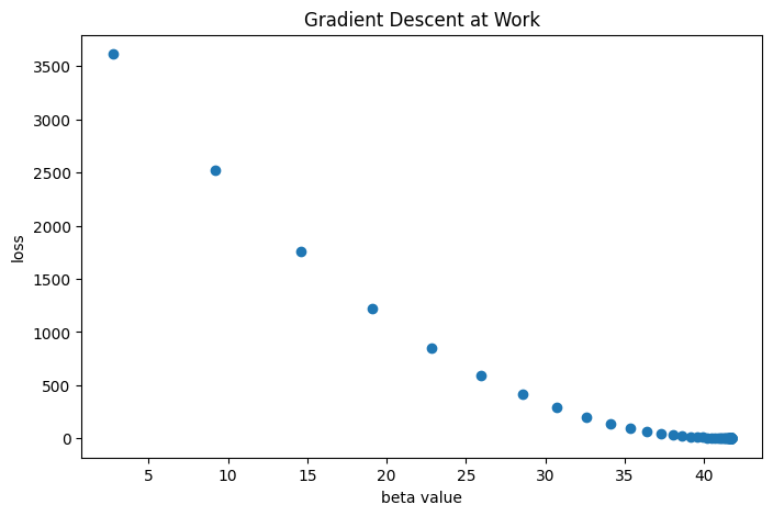
Here, we see that the algorithm converges at the estimated \(\beta\) little over 40. Let’s print out the best beta from gradient descent and the true parameter for comparison.
print(f"True parameter of the univariate model: {coef} \n \n ")
print(f"Best estimate from gradient descent: {beta} \n \n")
True parameter of the univariate model: 41.7411003148779
Best estimate from gradient descent: [[41.74109966]]
See that the estimate obtained from gradient descent is close to the true parameter.
Multivariate model
The gradient descent works similarly in case of multivariate model specification except that we’ll have a vector of partial derivatives. The multivariate model specified at the very begining is:
\[ \begin{aligned} Y_i = \alpha + \beta_1 X_{1i} + \beta_2 X_{2i} + \epsilon_i \\ MSE(\theta) = \frac{1}{m} (Y - X \theta)^{T}(Y - X \theta) \end{aligned} \]
I’ve expressed MSE in matrix form, where \(\theta\) incorportates the vector of parameters: \(\theta = [\alpha, \; \beta_1, \; \beta_2]^{T}\).
The gradient vector is given as: \[ \frac{\partial MSE}{\partial \theta} = \frac{1}{m} 2 X^{T}(Y - X \theta) \]
The gradient vector is of dimension \(3 \times 1\) and stacks all partials of MSE with respect to \(\alpha\), \(\beta_1\) and \(\beta_2\).
Let’s code the gradient descent algorithm and print out both the true parameters and their estimates.
# Use the gradient descent algorithm
m = X.shape[0]
y = y.reshape((m, 1))
theta = np.random.randn(3, 1)
eta = 0.1

for i in range(100):
    gradient = -2 / m * X.T @ (y - X @ theta)
    theta = theta - eta * gradient

# True coefficients
print(f"True coefficients: {np.hstack([10, coefficient])}")
print(f"Coefficients from gradient descent: {theta}")
True coefficients: [10. 40.71064891 6.60098441]
Coefficients from gradient descent: [[10.00156879]
[40.74650076]
[ 6.62076533]]Note that these coefficients are exactly similar to those obtained from the normal equation method. We can also make sure that we’ve done the estimation correctly by comparing the estimates with those obtained from built in module in sklearn used for purposes of estimating linear regression models.
# sklearn
reg = linear_model.LinearRegression(fit_intercept=True)
reg.fit(X, y)
best_theta_coef = reg.coef_
best_int_coef = reg.intercept_
best_theta_coef = np.concatenate([best_int_coef, best_theta_coef[:, 1:3].ravel()], axis = 0)
print(f"coefficients from sklearn: {best_theta_coef}")
coefficients from sklearn: [10.00156877 40.74650082 6.62076534]Not too bad!!
Standard Error
# ----------------------------------------------


# Standard errors


# ----------------------------------------------

# 1. Get the standard error of the regression

error = (X @ theta - y)
error_sq = error.T @ error
sigma_sq = 1 / (m -3) * error_sq
se_reg = np.sqrt(sigma_sq)
print(f"standard error of the regression is: {se_reg}")

# 2. get standard errors of the respective coefficients
var_cov = np.linalg.inv(X.T @ X) * sigma_sq
manual_se = np.sqrt(np.diag(var_cov))
print(f"standard errors of coefficients (manual estimation): {manual_se}")

# se from stats model
X_sm = sm.add_constant(X)   # add intercept
model = sm.OLS(y, X_sm).fit()

print(f"coefficients from statmodels: {model.params}")   # coefficients
print(f"standard errors from statmodels: {model.bse}")      # standard errors
standard error of the regression is: [[0.98562573]]
standard errors of coefficients (manual estimation): [0.03123574 0.03242909 0.03072431]
coefficients from statmodels: [10.00156877 40.74650082 6.62076534]
standard errors from statmodels: [0.03123574 0.03242909 0.03072431]