5 Standard Errors
Course: Causal Inference
Topic: Estimation of linear regression model and standard errors
Standard Errors
As previously mentioned, we start with a specification oriented towards the population and use a sample to estimate the population parameters. The \(\hat{\beta}\) are the sample estimates that inform us about the population parameters \(\beta\). In this sense, sampling variability – if you were to take say 1,000 samples from the population and re-estimate the parameter – will give you different estimates of \(\beta\). Just as the sample mean is a random variable with its own distribution, so is \(\hat{\beta}\). The standard error of \(\hat{\beta}\) plays the same role as the standard error of the mean, which we motivate below.
Consider the following example of mean height. Say, the population distribution is normal with mean 175 cm and standard deviation of 7.6 cm. You first take a sample of 1,000 individuals and estimate the mean height; then re-take the next sample, re-estimate the mean, and so on for 1,000 different samples. This will give you a distribution of mean height estimates, which will itself be normal with a variance driven entirely by sampling variability.
It is important to note that in practice you only ever have one sample – the simulation below is a thought experiment to build intuition for what would happen under repeated sampling. This is the frequentist conception of uncertainty.
By the Central Limit Theorem (CLT), the sampling distribution of the mean is: \[\hat{X} \sim \mathcal{N}\left(\mu,\ \frac{\sigma}{\sqrt{n}}\right)\] where \(\sigma\) is the population standard deviation (fixed but unknown in practice) and \(\frac{\sigma}{\sqrt{n}}\) is the standard error – the standard deviation of the sampling distribution of the mean, not of the population itself. Note the distinction: \(\sigma\) describes variability in individual heights; \(\frac{\sigma}{\sqrt{n}}\) describes variability in the estimate of the mean across repeated samples.
Let’s simulate height coming from a normal distribution with mean 175 cm and standard deviation 7.6 cm.
import numpy as np
import matplotlib.pyplot as plt
from sklearn.preprocessing import add_dummy_feature
from sklearn import linear_model
from scipy import stats

mean_store = []
iter = 10000
mean_height = 175
std_height = 7.6
n = 1000


for i in range(0, iter):
    height = np.random.normal(mean_height, std_height, n) # sample height from a normal distribution
    mean_store.append(height.mean())

# plot the histogram of mean height
mean_store = np.array(mean_store).ravel()

# overlay theoretical normal dist
x_space = np.linspace(mean_store.min(), mean_store.max(), 1000)
theo_nd = stats.norm.pdf(x_space, mean_height, std_height/np.sqrt(n))

plt.figure(figsize=(8, 5))
plt.hist(mean_store, bins=30, color='steelblue', edgecolor='black', alpha=0.3, density='True')
plt.plot(x_space, theo_nd, color = 'red', linewidth = 2, label = 'Theoretical Dist.')
plt.title(f'Distribution of mean height from {iter} different samples')
plt.xlabel('mean height')
plt.ylabel('density')
plt.legend()
plt.grid(False)

print(f'average of mean height is {mean_store.mean().round(4)} and std is {mean_store.std().round(4)}')
average of mean height is 174.997 and std is 0.2402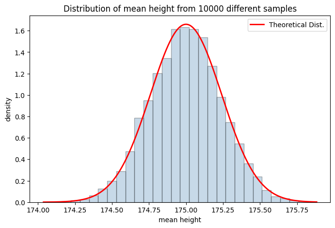
It is clear that the standard deviation of the mean height depends on: i) the standard deviation of the population height; and ii) n – the number of observations. The standard deviation of the mean height will be lower if the population standard deviation is lower (meaning that height is relatively more homogeneous). Next, one can lower it by increasing the sample size.
Just as the sample mean has a measure for deviation due to sampling variability (standard deviation), \(\hat{\beta}\) too has a measure that we know as standard errors. Simply put, the standard errors measure how fluctuating the estimates of \(\beta\) can be given different samples.
Right off the start, it should be mentioned that reported standard errors are mostly incorrect. This could be due to several unknown reasons including the functional form of the specified model. But rather than dwelling on why the reported standard errors are incorrect, I want to discuss some known ways to fix the standard errors.
First, (recall) we start with the assumption on the error term. We discussed the i.i.d. assumtion of the error term. Again, the i.i.d. assumption states that error term are independent and identically distributed. The former means that errors are not correlated, whereas the latter means that errors are extracted from the same distribution with the same mean and variance.
Under the i.i.d. assumption, errors are homoskedastic. Estimation of standard errors take the following steps.
First estimate the regression standard error as: \(\sigma_{reg}^2 = \frac{1}{n}\epsilon^{T} \epsilon\).
The standard error of estimates then is: \(\sqrt{Var(\hat{\beta})} = (X^{T}X)^{-1} \times \sigma_{reg}\), where \(X^{T}X\) is the variance-covariance matrix with variance terms in the diagonal.
However, both of these assumptions (identical and independently distributed) will mostly likely fail in practice. This means that we’d need to adjust the standard errors appropriately.
Let’s take a classic example between education and earnings. We’ll also consider ‘ability’ as a control variable in the DGP. Of course, this is only a simulation exercise to clarify the context of standard errors.
# 1. generate ability score with a mean of 50 and sd of 20.
m = 10000
ability = np.random.normal(50, 20, m)
ability_scaled = (ability - ability.mean()) / ability.std() # ability scaled

# plot histogram of ability score
plt.figure(figsize=(8,5))
plt.hist(ability, bins=30, color='steelblue', edgecolor='black', alpha=0.3)
plt.title('Distribution of ability')
plt.xlabel('ability score')
plt.ylabel('frequency')

# 2. education is positively dependent on ability
educa = 7 + 0.1 * ability + np.random.normal(0, 4, m)
educa[educa<0] = 0
educa_scaled = (educa - educa.mean()) / educa.std() # education scaled
#plt.hist(educa)

# 3. generate income
# Income comes from distribution with varying standard deviation
# this marks heteroskedasticity
error_term = np.random.normal(0, 500 + (200*educa))

# generate income using the following DGP
income = 40000 + 10000 * educa_scaled + 700 * ability_scaled + np.array(error_term).ravel()
true_coefficients = np.array([40000, 10000, 700])

# scatter plot between schooling and education
plt.figure(figsize=(8,5))
plt.scatter(educa, income)
plt.title('Scatter plot of education and income')
plt.grid(True, linestyle ='dashed', alpha = 0.3)
plt.xlabel('Schooling')
plt.ylabel('Earnings')

# scatter plot between schooling and error
error_true = income - (40000 + 10000 * educa_scaled + 700 * ability_scaled)

plt.figure(figsize=(8, 5))
plt.scatter(educa, error_term, alpha = 0.3, color = 'red')
plt.title('Relationship between schooling and error term \n using the true parameters')
plt.xlabel('Schooling')
plt.ylabel('Error')
plt.grid(True, linestyle='dashed')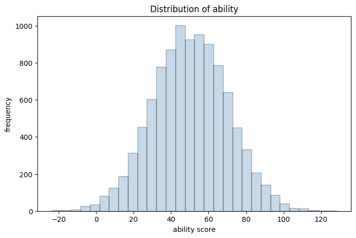
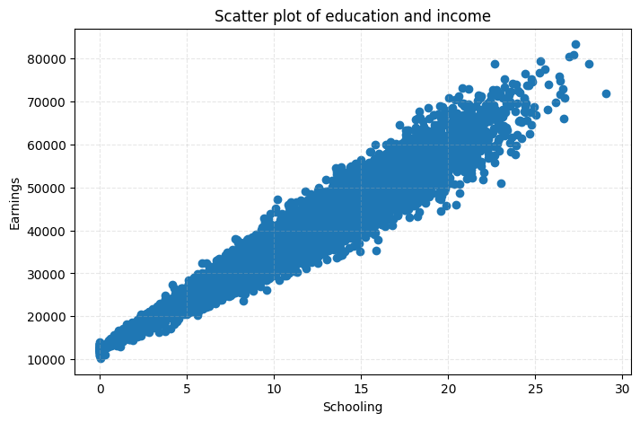
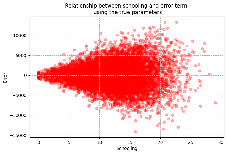
The plot above shows that although there exist a positive correlation between schooling and earnings, variation in earnings is higher for greater values of education. Using the true coefficients (we have these since this is a simulated DGP) we extract error and plot the relationship between schooling and errors. Here, we see a funnel shaped scatter plot with the mean of error aligned at 0. This simple example breaks the homoskedasticity assumption. The main point is that the estimation of standard errors need to reflect the fact that error term comes from distribution with different variances. We now have what is known as heteroskedasticity.
Let’s start with regression estimates using the gradient descent.
# features
X = np.concatenate((educa_scaled.reshape(m,1), ability_scaled.reshape(m,1)), axis = 1)
# Note: no need to scale the features as they already are scaled
X = add_dummy_feature(X) # intercept term
y = income.reshape((m, 1))
p = X.shape[1]           # number of features

# initialize theta
theta = np.random.uniform(0, 1, p).reshape((p, 1))
# learning rate
eta = 1e-2
# number of iterations
epochs = 2000

for i in range(0, epochs):

    # get the gradient and adjust theta against the gradient using the learning rate
    gradient = -2/m * X.T@(y - X@theta )
    theta = theta - eta*gradient


# Use sklearn module to check
reg = linear_model.LinearRegression(fit_intercept=False)
reg.fit(X, y)
print(f'The estimates from sklearn is: {reg.coef_.round(4)}')
print(f'The estimates from manual GD is: {theta.reshape((1, 3)).round(4)}')
The estimates from sklearn is: [[39987.2777 9991.4859 695.5676]]
The estimates from manual GD is: [[39987.2777 9991.4859 695.5676]]We are simply running gradient descent in the code above. This should be familiar to you from previous lectures. Now, we’d want to move on to the standard errors to determine precision of these estimates. First, let’s explore the graphical relationship between education and residuals. Note that I’ve distinguised error vs. residual – the former is what you get from using true coefficients (you never see this in practice), while the latter uses the estimates.
# Get residuals (note that we are using the estimated thetas)
residual = y - X @ theta
plt.figure(figsize=(8,5))
plt.scatter(educa, residual, alpha = 0.3, color='red')
plt.title('Relationship between education and residuals')
plt.xlabel('education')
plt.ylabel('residuals')
plt.grid(True, linestyle='dashed')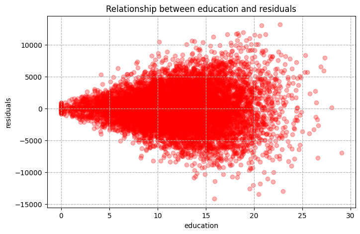
As you can see we’ve got a funnel shaped relationship between education and residual, again signaling heteroskedasticity. This is precisely coming from differing variance of error term based on education. This won’t affect the estimates but will affect the standard errors. Note that there are many tests for homoskedasticity vs heteroskedasticity. But in practice, the case of homoskedasticity almost always fails. The simple way to see it is to plot the residuals with the variable of concern. If you have a funnel looking shape, then you’ve got the case of heteroskedasticity.
First, let’s do some benchmarking by estimating the standard errors under the homoskedasticity assumption – error terms have the same variance (which is incorrect in this case and in practice).
# 1. Get the standard error of the regression
error = (X @ theta - y)
error_sq = error.T @ error
sigma_sq = 1 / (X.shape[0] -3) * error_sq
se_reg = np.sqrt(sigma_sq)
print(f"standard error of the regression is: {se_reg} \n \n")
# 2. get standard errors of the respective coefficients
var_cov = np.linalg.inv(X.T @ X) * sigma_sq
manual_se = np.sqrt(np.diag(var_cov))
# compare it with standard errors from statsmodels
import statsmodels.api as sm
# se from stats model
X_sm = sm.add_constant(X) # add intercept
model = sm.OLS(y, X_sm).fit()
print(f"The estimates from statmodels: {model.params.round(4)}") # coefficients
print(f'The estimates from sklearn is: {reg.coef_.round(4)}')
print(f'The estimates from manual GD is: {theta.reshape((1, 3)).round(4)} \n \n')
print(f"standard errors from statmodel under homoskedasticity: {model.bse.round(4)}") # standard errors
print(f"standard errors (manual estimation) under homoskedasticity: {manual_se.round(4)} \n \n")standard error of the regression is: [[3048.97689642]]
The estimates from statmodels: [39987.2777 9991.4859 695.5676]
The estimates from sklearn is: [[39987.2777  9991.4859   695.5676]]
The estimates from manual GD is: [[39987.2777  9991.4859   695.5676]]
standard errors from statmodel under homoskedasticity: [30.4898 33.9277 33.9277]
standard errors (manual estimation) under homoskedasticity: [30.4898 33.9277 33.9277]
Now that we have estimated standard errors under the homoskedasticity assumption let’s see how we can fix this. Before we move on, I want to reiterate that the origin of heteroskedasicity is due to error terms coming from the distribution of different variance. In that regard, we want to account for this in our estimation of standard errors.
To do so, we’ll use a sandwich method, which you should’ve heard from you previous classes. So what does it entail? Basically, we’d want to form weights using the size of the error term.
Let’s just derive the sandwich estimator:
\[\begin{align} \hat{\beta} = (X^{T}X)^{-1}X^{T}Y \\ \hat{\beta} = (X^{T}X)^{-1}X^{T}(X\beta + \epsilon) \\ \hat{\beta} = \beta + (X^{T}X)^{-1}X^{T}\epsilon \end{align}\]
The end line is the starting point. Note that \(Var(a)=0\) and \(Var(ax) = a^{2}Var(x)\), where \(a\) is a constant and \(x\) is a random variable. Let’s then take the variance of \(\hat{\beta}\):
\[\begin{align} Var(\hat{\beta}) = Var((X^{T}X)^{-1}X^{T}\epsilon) \\ = (X^{T}X)^{-1}Var(X^{T}\epsilon)(X^{T}X)^{-1} \\ = (X^{T}X)^{-1}X^{T}Var(\epsilon)X(X^{T}X)^{-1} \\ = (X^{T}X)^{-1}X^{T} \Omega X(X^{T}X)^{-1} \end{align}\]
Here, \(\Omega\) is the scaling term and it is \(\epsilon\epsilon^{T}.I\), which is a \(n \times n\) diagonal matrix. We don’t observe this, so replace this with the sample counterpart \(\hat{\Omega} = \hat{\epsilon}\hat{\epsilon}^{T}I\). Notice that under the case of homoskedasticity \(\Omega = \sigma^2 I\), which collapses \(Var{\hat{\beta}}\) to \((X^{T}X)^{-1} \sigma^2\). This is what we used to estimate standard errors under homoskedasticity.
Let’s estimate the standard errors accounting for heteroskedasicity. I’m going to divide this into bun and stuffing part as I write the code.
bun = np.linalg.inv(X.T@X)
omega = np.diag((residual**2).ravel()) # n * n diagonal matrix
stuff = X.T @ omega @ X

# get the variance covariance matrix
var_cov = bun @ stuff @ bun
robust_se = np.sqrt(np.diag(var_cov))
print(f'heteroskedasticity robust standard error: {robust_se.round(4)}')
print(f'se under homoskedastic assumption: {manual_se.round(4)}')

# robust se using sm
model2 = sm.OLS(y, X).fit(cov_type='HC0')
print(f'standard errors from stats model under heteroskedasticity: {model2.bse.round(4)}')
heteroskedasticity robust standard error: [30.4852 36.4511 34.2139]
se under homoskedastic assumption: [30.4898 33.9277 33.9277]
standard errors from stats model under heteroskedasticity: [30.4852 36.4511 34.2139]If you compare the standard errors under homoskedasticity versus heteroskedasticity, you will see that standard errors under heteroskedasticity are larger, particularly for the education estimate.
Note that there are various forms of heteroskedasicity robust standard error including “HC1”, “HC2”, and “HC3”. Here, we’ve used the “H0” type – you can dig deeper according to your need.
Let’s now discuss the case where error terms are not independent and are correlated. One can think of this in a geospatial form – the unexplained portion of income for people living in a particular area can be correlated. For example, if you have people living in Des Moines, Iowa and NYC in your sample, you’ll probably think that income is spatially correlated due to local market conditions, taste, cost of living and other unobserved factors attributing to spatial clustering.
In the following simulation exercise, we’ll incorporate this cluter-type correlation in the error terms. Specifically, we’ll build error as:
\[\begin{equation} \epsilon_{ic} = u_{c} + v_{i} \end{equation}\]
Essentially, the error term consists of: i) \(u_c\) – the cluster specific shock (all units within a specific cluster gets the same value); and ii) individual specific term. Both \(u_c\) and \(v_i\) will come from a normal distribution with mean 0 and standard deviation 3,000 and 1,000, respectively.
# number of clusters
nc = 50

# number of units within cluster
ni = 200

# total number of units
m = nc * ni

# get the cluster shock
cluster_shock = np.random.normal(0, 3000, nc)
cluster_index = np.repeat(np.linspace(1, nc), ni).astype('int')
u_shock = cluster_shock[cluster_index-1]

# get the individuals shock
# in this case cluster shock dominates individual shock
v_shock = np.random.normal(0, 1000, m)

error = u_shock + v_shock
Let’s estimate the model and plot the relationship between education and residuals by some clusters.
X = np.concatenate((educa_scaled.reshape((m, 1)), ability_scaled.reshape((m,1))), axis=1)
X = add_dummy_feature(X)
y_c = 40000 + 10000 * educa_scaled + 700 * ability_scaled + error.ravel()
y_c = y_c.reshape((m, 1))

# initialize theta
theta = np.random.uniform(0, 1, p).reshape((p, 1))
# learning rate
eta = 1e-2
# number of iterations
epochs = 20000

for i in range(0, epochs):
    # get the gradient and adjust theta against the gradient using the learning rate
    gradient = -2/m * X.T@(y_c - X@theta)
    theta = theta - eta*gradient

print(theta)

resid_clus = y_c - X@theta


# then re-generate income

error_clus = income - (40000 + 10000 * educa_scaled + 700 * ability_scaled)
plt.figure(figsize=(8,5))
plt.scatter(educa[cluster_index==1], resid_clus[cluster_index==1], color = 'red', alpha = 0.3, label='Cluster 1')
plt.scatter(educa[cluster_index==10], resid_clus[cluster_index==10], color = 'blue', alpha = 0.3, label='Cluster 10')
plt.scatter(educa[cluster_index==20], resid_clus[cluster_index==20], color = 'green', alpha = 0.3, label='Cluster 20')
plt.legend()
plt.title('Relationship between schooling and residuals \n by some chosen cluster')
plt.xlabel('schooling')
plt.ylabel('residuals')
[[40216.91715969]
[ 9940.69952697]
[ 754.42493803]]
Text(0, 0.5, 'residuals')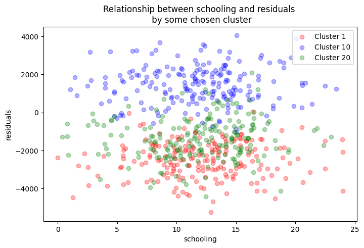
In the figure above, we see that residuals across different clusters are grouped at certain residual values. This depicts the clustering problem. Now, we need to adjust our the standard errors to account for this kind of clustering. The variance now takes the form:
\[\begin{equation} Var(\hat \beta) = (X^{T}X)^{-1} \bigg(\sum_{c=1}^{G} X^{T}_c \epsilon_c \epsilon^{T}_c X_c \bigg) (X^{T}X)^{-1} \end{equation}\]
Let’s estimate this!!
bun = np.linalg.inv(X.T@X)
stuff = np.zeros(X.shape[1]*X.shape[1]).reshape((X.shape[1], X.shape[1]))

for i in range(1, nc+1):

    X_c = X[cluster_index==i]
    res_c = resid_clus[cluster_index==i]

    mid = X_c.T@res_c@res_c.T@X_c
    stuff += mid

var_cov_clus = bun@stuff@bun
se_clus = np.sqrt(np.diag(var_cov_clus))


# small sample correction term
correction = ((nc/(nc-1)) * (m-1)/(m-p))
var_cov_clust_corr = var_cov_clus * correction
se_clus_correct = np.sqrt(np.diag(var_cov_clust_corr))

model_clus = sm.OLS(y_c, X).fit(cov_type='cluster', cov_kwds={'groups': cluster_index})
model_noclus = sm.OLS(y_c, X).fit()

print(f'Clustered standard errors (not small sample corrected): {se_clus.round(4)}')
print(f'Clustered se corrected for small sample: {se_clus_correct.round(4)}')
print(f'Clustered standard error from statsmodel: {model_clus.bse.round(4)}')
print(f'standard error without clustering from statsmodel: {model_noclus.bse.round(4)}')
Clustered standard errors (not small sample corrected): [452.4901 38.7462 35.9821]
Clustered se corrected for small sample: [457.1298 39.1435 36.3511]
Clustered standard error from statsmodel: [457.1298 39.1435 36.3511]
standard error without clustering from statsmodel: [33.5377 37.3193 37.3193]We’ve now computed the clustered standard errors and compared it with those from statsmodel. They are exactly the same. However, clustered standard errors are larger compared to non-clustered standard errors.
Bootstrapped standard errors
Bootstapping can lead to a convenient way of obtaining standard errors. The bootstrapping process assumes the sample as the population and performs resampling \(k\) number of times from the population (with replacement). For each re-sampling we estimates the coefficients. With this process, you’ll then have \(k\) number of estimates. Then the standard error is simply the standard deviation of the estimates.
import random

rep = 199
# learning rate
eta = 1e-2
# number of iterations
epochs = 20000

for k in range(0, rep):

    boot_index = np.random.choice(X.shape[0], size=X.shape[0], replace=True).astype('int')
    boot_index = np.array(boot_index) - 1
    X_boot = X[boot_index]
    y_boot = y_c[boot_index]

    # initialize theta
    theta = np.random.uniform(0, 1, p).reshape((p, 1))

    for i in range(0, epochs):
    # get the gradient and adjust theta against the gradient using the learning rate
        gradient = -2/X_boot.shape[0] * X_boot.T@(y_boot - X_boot@theta)
        theta = theta - eta*gradient

    if k == 0:
        theta_store = theta.ravel()
    else:
        theta_new = theta.ravel()
        theta_store = np.vstack((theta_store, theta_new))

    #print(f'Rep {k} estimate: {theta}')

plt.figure(figsize=(8,5))
plt.hist(theta_store[:,1], bins = 30, color='steelblue', edgecolor='black', alpha=0.3)
plt.xlabel('Schooling estimates')
plt.ylabel('Frequency')
plt.title(f'Histogram of bootstrapped estimate \n from {rep} replications.')


boot_se = theta_store.std(axis=0)
print(f'bootstrapped non-clustered version of se: {boot_se.round(4)}')
print(f'standard error without clustering from statsmodel: {model_noclus.bse.round(4)}')
bootstrapped non-clustered version of se: [30.6567 37.8813 38.6351]
standard error without clustering from statsmodel: [33.5377 37.3193 37.3193]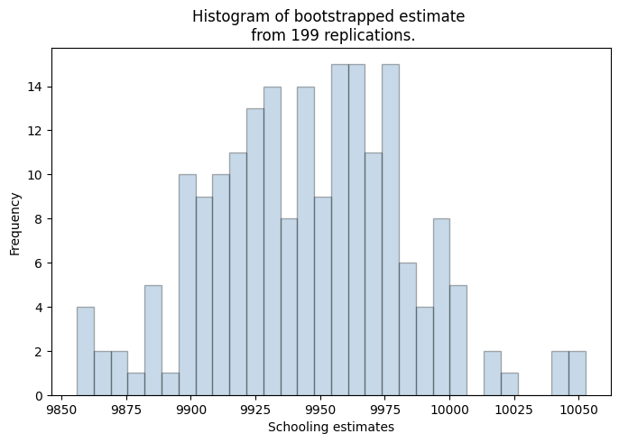
There you have it – the bootstrapped version of the standard errors. Note that we’ve not accounted for the clusters and one can do that by sampling clusters (with replacement) rather than units.